

Every edge device that talks wirelessly is making a real estate decision. Spectrum is finite, regulated, and crowded, and the band you choose shapes everything downstream: range, throughput, power budget, antenna size, interference exposure, and whether you need a license at all. Pick well, and your deployment hums along for years; pick poorly, and you’re chasing intermittent link failures across a field of duty-cycled sensors at 2 a.m.
For a business, that is not an abstract engineering concern; it is the difference between a project that ships and one that quietly bleeds money. The band decision drives what a deployment costs to install, how often a technician has to visit, whether the data arrives reliably enough to act on, and whether a competitor with the right radio can do the same job for a third of the price. A warehouse that picks the wrong wireless for its inventory tags, a farm that streams video no link can carry, or a property manager who wires every camera when a single sub-GHz mesh would have served: these are ordinary, expensive mistakes, and they all trace back to a spectrum choice made without understanding the tradeoffs. This article exists to make that choice legible.
This post is a practical tour of the spectrum available to private and commercial entities in the United States, organized by band, with an emphasis on what each slice is actually good for at the edge and what it lets a business do that it couldn’t do affordably before. The regulatory framing is FCC-centric, but the engineering trade-offs are universal. For a sobering look at just how contested this real estate is, keep the NTIA’s full allocation chart (Figure 1) open in another tab as you read; every band discussed below is a thin sliver of it.
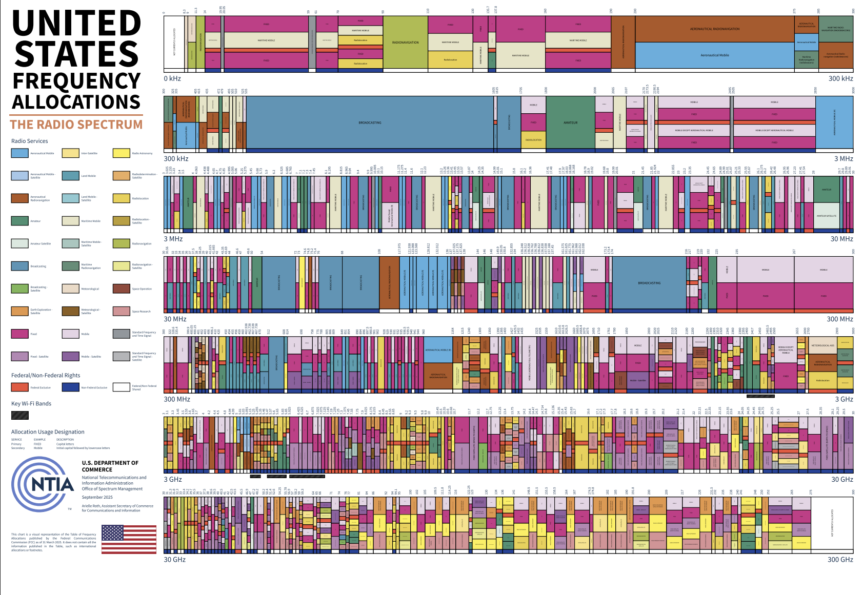
Figure 1. The United States Frequency Allocations chart (NTIA, September 2025). Every technology in this article occupies a narrow slice of this map, shared with incumbents that predate it. Source: NTIA / Wikimedia Commons (public domain, U.S. Government work).
1 Bottom Line Up Front: What This Actually Means for a Business
Before the physics and the band names, here is the part that lands on a budget. The reason any of this matters to an ordinary company comes down to four levers that a spectrum decision moves directly, and everything technical that follows serves to pull one of them.
It moves the cost from a subscription to an asset. The default way to connect a remote device is via a cellular plan, which bills per device per month indefinitely. Most of the unlicensed technologies in this article replace that recurring line item with hardware you buy once and own. A hundred sensors on a private LoRaWAN or HaLow network cost roughly the same to run whether they send one message a day or a thousand, and nothing arrives on next month’s invoice. For a deployment that will last for years, the crossover math is stark and usually favors owning the network.
It moves cost out of the truck roll. The most expensive part of most edge deployments is not the device; it is the human who installs and services it. Every choice that lets a node run longer without a visit, whether that is a low-power radio, a solar power budget sized for the worst week of winter, or a mesh that self-heals when one node drops, is money not spent sending someone into the field. The cheapest node really is the one nobody has to drive out to. This is also where the RF and sensing approaches quietly beat cameras on operating cost: an optical lens is a maintenance item, and an ever-growing wall of cameras means an ever-growing chore of cleaning, defogging, and clearing the spider webs, dust, pollen, and bird droppings that blind a lens and generate service calls. An RF antenna has no lens to foul; it is effectively maintenance-free, works through the same grime and weather that degrade an optical sensor, and does not multiply the janitorial burden every time you add a node. At scale, the difference between sensors you must keep clean and sensors you can forget is a real line item in the budget.
It turns physical questions into data cheaply. A great deal of what businesses want to know is physical: where is the space occupied, how fast is the traffic moving, where is the equipment, and did something cross the fence? The sensing bands turn those questions into a feed for tens of dollars per point, in any weather, often without the privacy overhead that cameras carry. That reframes problems that used to need staff or guesswork as things you simply measure. Fused across the entire operation, those feeds give analysts a continuous account of how every location performs, from the production line to the sales floor to the loading dock, and how efficiently each vertical hands off to the next.
It buys reliability and control. On a shared, congested, or carrier-owned network, a business is renting performance that cannot be guaranteed. Owning the right slice of spectrum, whether a quiet sub-GHz mesh, a private CBRS cell, or a directional backhaul link, means the operation controls its own uptime and its own data path. For anything where an outage stops work or where the data is sensitive, that control is often worth more than raw connectivity.
None of these levers require a business to become a wireless expert. They require deliberately choosing which of the four a given deployment is really about, and then picking the band that pulls it the hardest. The rest of this article is the map from levers to bands: the physics and constraints that narrow the field, a band-by-band tour of what each slice does best, and a decision table at the end that turns it all into a lookup.
2 The Physics You Can’t Negotiate With
Before the band-by-band tour, three rules govern everything:
Lower frequency propagates farther and penetrates better. A 900 MHz signal will punch through foliage and drywall that stops 5 GHz cold; free-space path loss scales with frequency, and material attenuation gets worse as wavelength shrinks. This is why long-range, low-power IoT lives almost entirely below 1 GHz.
Higher frequency carries more data. Wider channels are easier to find up high; there’s simply more spectrum available at 5 GHz than at 900 MHz, and vastly more at 60 GHz. Throughput follows channel width.
Power and duty cycle are regulated, not just engineered. Unlicensed bands have EIRP limits, and some have duty-cycle or listen-before-talk requirements. Your link budget is bounded by the FCC before it’s bounded by your amplifier.
Everything below is a different point on the triangle of range, throughput, and regulatory freedom.
3 The Tyranny of SWaP-C
Borrowed from the defense and aerospace world, SWaP-C (Size, Weight, Power, and Cost) is the four-axis vise that every edge device gets squeezed in. The term earned the word “tyranny” honestly: these four constraints are coupled, and improving one almost always degrades another. At the edge, SWaP-C isn’t a procurement checklist; it’s the physics of your deployment expressed in dollars, watts, and grams.
Consider how the coupling works in an RF context:
Power drives everything else. A radio that draws 2 W average instead of 200 mW doesn’t just cost you 1.8 W; it costs you a larger battery, a larger solar panel, a beefier charge controller, a bigger enclosure to hold it all, and a heavier mast or mount to carry it. Power consumption cascades through the entire bill of materials with a multiplier attached. This is why the difference between a Wi-Fi radio idling at hundreds of milliwatts and a HaLow or LoRa radio sleeping at microamps isn’t an incremental spec-sheet win; it can be the difference between a shoebox-sized node and a Pelican case with a 100 W panel bolted to it.
Size and weight constrain antennas, and antennas are your link budget. Sub-GHz’s propagation advantage comes with a tax: a quarter-wave antenna at 915 MHz is about 8 cm, and efficient high-gain sub-GHz antennas get physically large, while a 60 GHz array fits on a postage stamp. Every band choice is implicitly an antenna-size choice, and antenna size is enclosure size, wind load, mounting hardware, and visual signature.
Cost is the constraint that compounds. Unit cost matters, but at the edge, deployed cost is the real number: the radio, the power system, the enclosure, the mount, the truck roll to install it, and the truck rolls to service it. A $40 radio that needs a $300 solar power system and quarterly battery swaps is not a $40 radio; the cheapest node is usually the one you never have to visit.
The tyranny is that there is no escape, only informed trades. Duty cycling buys you power at the cost of latency and availability (a node that wakes on motion is blind while it boots); higher frequency buys you small antennas at the cost of range; more transmit power buys you link margin at the cost of everything in the power cascade above. The discipline SWaP-C imposes is valuable precisely because it forces you to decide, explicitly, what your deployment actually needs before the field decides for you.
4 Shore Power vs. Solar and Batteries: The First Fork in the Road
Before you pick a band, a protocol, or a chipset, answer one question: does this node have a wall outlet, or does it live off the grid? More than any other single factor, the answer partitions the entire solution space.
4.1 The shore power regime
If a node has mains power (PoE from a switch, an outdoor outlet, or a light pole with a photocell tap), the power axis of SWaP-C effectively collapses, and with it, most of the tyranny. You can run radios that would be unthinkable on batteries: 5/6 GHz Wi-Fi access points burning 10–25 W, CBRS small cells at 20 W and up, 60 GHz backhaul terminals, and always-on compute doing local inference. Latency and availability are free because nothing needs to sleep; video can stream continuously rather than trigger on events. Your design conversation shifts almost entirely to throughput, coverage, and spectrum coexistence.
PoE deserves special mention as the edge deployer’s best friend: 802.3af/at/bt delivers 13–71 W over the same cable that carries your data, giving you a single-run install with centralized power backup at the switch. If you can reach a node with 100 m of Ethernet, that is nearly always the right answer; the “wireless” decision then applies only to links you genuinely cannot cable.
4.2 The solar and battery regime
The moment a node goes off-grid, the power system becomes the dominant engineering problem and frequently the dominant line item. The radio is no longer the design center; the energy budget is, and everything is derived from it:
Sizing is set by your worst day, not your average day. Solar design starts with worst-case insolation, which, for the continental US, typically means December, when peak sun hours can drop to 3–4 per day even in the Sun Belt, and far fewer under extended cloud cover. A node that draws 1 W on average needs roughly 24 Wh/day, which means a panel sized to harvest that in 3 sun hours (with charge losses, call it a 15–20 W panel minimum) and a battery bank sized for 3–5 days of autonomy through weather. Every watt of average draw translates to roughly 15–20 W from the panel and 75–120 Wh from the battery once you apply real-world margins.
Chemistry and thermal reality matter. LiFePO4 has become the default for fixed solar nodes, offering safety, long cycle life, and tolerance of partial charge, but it won’t charge below freezing without heating or charge cutoffs. Lithium-ion 18650-class packs offer better energy density where weight matters; lead-acid still appears where cost dominates and weight doesn’t. Whatever the chemistry, your battery is the component most sensitive to the enclosure’s thermal design and the one whose degradation quietly shortens your maintenance interval.
Duty cycling becomes architecture, not optimization. Off-grid nodes push you toward radios and patterns that shore-powered nodes never consider: wake-on-motion via PIR sensors, scheduled wake windows managed by external power controllers, LoRa’s seconds-per-day airtime, and HaLow’s target wake time (TWT) mechanics. The protocol stack and the power system co-design each other.
4.3 How the fork drives the band choice
This is why the power source belongs in the spectrum decision, not downstream of it. The regimes map to bands with striking consistency (Table 1).
Table 1. Power regime as a determinant of band and technology choice.
| Power regime | Natural fits | Fights physics |
|---|---|---|
| Shore power / PoE | 5/6 GHz Wi-Fi, CBRS private LTE/5G, 60 GHz backhaul, continuous video | — |
| Solar + battery, generous (50 W+ panel) | HaLow mesh, duty-cycled video, LoRaWAN gateways, cellular routers | Always-on 5 GHz APs, small cells |
| Solar + battery, minimal (<10 W panel) | LoRaWAN end devices, NB-IoT/LTE-M, deep-sleep HaLow clients | Anything streaming, anything always-listening |
| Battery only, no harvest | BLE beacons, LoRa sensors, event-driven telemetry | Any IP-native always-on radio |
A hybrid pattern appears frequently in well-designed systems: shore-powered aggregation points (a PoE-fed HaLow access point or a LoRaWAN gateway in a building) serving constellations of solar- or battery-powered field nodes. Put the power-hungry, always-on infrastructure where power is cheap, and let the edge devices spend their precious milliwatt-hours only on their own traffic; the topology of your network should mirror the topology of your power.
5 Sub-GHz Unlicensed: The Long-Haul Workhorses
5.1 902–928 MHz (US ISM Band, Part 15)
This 26 MHz slice is the crown jewel of unlicensed long-range communication in the Americas. Under FCC Part 15.247, frequency-hopping and digitally modulated systems can transmit up to 1 W of conducted power (up to +36 dBm EIRP with antenna gain) with no duty-cycle restriction, a significant advantage over the European 868 MHz band, which imposes duty-cycle limits as low as 1%.
For a business, this band is where wireless stops being a recurring bill and becomes an owned asset. A farm, quarry, marina, or sprawling facility that would otherwise pay a cellular carrier per device, per month, forever can instead stand up its own sub-GHz network once and run thousands of sensors or a property-wide camera mesh on it for the cost of the hardware. That is the difference between an operating expense that scales with every device you add and a capital expense you amortize.
Three major technology families share this band, and they do not always coexist gracefully:
LoRa and LoRaWAN use chirp spread spectrum to achieve remarkable receiver sensitivity, with links closing at −137 dBm or better. Optimal uses: telemetry, sensor backhaul, metering, asset tracking, and anything where a few hundred bytes per message and multi-kilometer range matter more than latency or throughput. A LoRaWAN gateway with an SX1302-class concentrator can serve thousands of devices across a metro area. What LoRa is not: a video pipe, a voice channel, or a low-latency control link.
Wi-Fi HaLow (802.11ah) is the newest serious tenant and arguably the most interesting for edge computing. HaLow brings genuine IP networking to sub-GHz: real TCP/IP and real throughput measured in megabits per second. With 1–8 MHz channel widths, HaLow delivers anywhere from a few hundred kbps to tens of Mbps at ranges of a kilometer or more, and current-generation chipsets support multi-hop mesh topologies as well as conventional point-to-multipoint links. Optimal uses: camera backhaul at modest bitrates, mesh networking across a campus or rural property, and IP connectivity to devices that would otherwise need cellular connectivity. A 1080p H.264 stream at low framerate fits comfortably in a HaLow link budget, something no other unlicensed sub-GHz technology can claim.
Legacy FHSS systems (SCADA radios, older proprietary telemetry links, cordless phones, and baby monitors) still populate this band, along with significant noise from RFID readers near logistics facilities.
The coexistence challenge is real. If you run both a LoRaWAN gateway and a HaLow mesh at the same site, an increasingly common architecture, plan your channels deliberately. Park LoRaWAN on the standard US915 sub-bands, place HaLow channels away from them, and, where possible, physically separate antennas vertically. Both radios are in the same 26 MHz; pretending otherwise costs you packet error rate.
5.2 433 MHz (Limited in the US)
In the US, 433.05–434.79 MHz falls under Part 15.231 with severe restrictions: periodic transmissions only and very low power. It’s the domain of key fobs, tire pressure sensors, and simple remote controls. In ITU Region 1 (Europe, Africa), 433 MHz is a legitimate ISM band with broader use; for US deployments, treat it as unavailable for anything serious.
6 2.4 GHz: The Crowded Commons
The 2400–2483.5 MHz ISM band is the most heavily used spectrum on Earth: Wi-Fi (802.11b/g/n/ax), Bluetooth and BLE, Zigbee, Thread, proprietary protocols, and microwave ovens all pile in.
Its virtues are universality and silicon cost. A 2.4 GHz radio costs pennies, works identically worldwide, and every phone on the planet can talk to it. Optimal edge uses: BLE for provisioning, local configuration, beacons, and short-range sensor connections. Thread)/Zigbee for dense, low-power mesh in buildings (smart lighting, HVAC sensors, and occupancy detection), where 802.15.4’s low duty cycle and mesh healing shine. 2.4 GHz Wi-Fi for devices that need real throughput and must work through a couple of walls.
The pathology of 2.4 GHz is congestion. In an apartment building or dense office park, the noise floor can be brutal; design for retries, and don’t put anything latency-critical here if you can avoid it.
7 5 GHz and 6 GHz: Throughput Territory
7.1 5 GHz (U-NII-1 through U-NII-4)
Roughly 5150–5895 MHz, carved into sub-bands with differing power limits and DFS (Dynamic Frequency Selection) requirements. DFS matters at the edge: in U-NII-2 bands, your device must vacate a channel if it detects radar, which can cause 60-second outages during channel availability checks. For fixed outdoor point-to-point links, U-NII-1 and U-NII-3 (no DFS) are the pragmatic choices.
Optimal uses: high-throughput local links, Wi-Fi backhaul between buildings, video streaming from edge cameras to a local recorder, and point-to-point bridges up to a few kilometers with directional antennas. The 5 GHz band remains the default answer for “I need tens to hundreds of Mbps, and I have near line of sight.”
7.2 6 GHz (U-NII-5 through U-NII-8)
The FCC’s 2020 opening of 5925–7125 MHz added 1200 MHz of unlicensed spectrum, the largest expansion in Wi-Fi history. Three device classes matter: Low Power Indoor (LPI) devices operate indoors without coordination. Very Low Power (VLP) devices can operate anywhere at reduced power. Standard Power devices, including those for outdoor use, require an Automated Frequency Coordination (AFC) system to protect incumbent microwave links.
For edge deployments: 6 GHz Wi-Fi 6E/7 is superb for high-density indoor environments (clean spectrum, wide channels, and multi-gigabit throughput), and AFC-coordinated standard-power operation is opening up serious outdoor fixed-wireless use. Propagation is slightly worse than 5 GHz, so this is a capacity play, not a range play.
8 CBRS (3550–3700 MHz): Private Cellular for the Rest of Us
The Citizens Broadband Radio Service is the most consequential spectrum innovation of the past decade for private networks. It’s a three-tier sharing framework: federal incumbents (primarily Navy radar) at the top, Priority Access License (PAL) holders in the middle, and General Authorized Access (GAA) users (that’s you, for free) at the bottom, all coordinated dynamically by Spectrum Access Systems (SAS) operated by companies like Google and Federated Wireless.
What CBRS enables is private LTE and private 5G. Instead of Wi-Fi’s contention-based access, you get scheduled, SIM-authenticated, carrier-grade wireless on spectrum you don’t have to buy at auction. Optimal uses: large industrial campuses, ports, mines, warehouses, and agricultural operations where you need deterministic performance, seamless mobility across hundreds of acres, and a better security posture than a PSK Wi-Fi network. AGV fleets, push-to-talk, and mobile edge devices roaming a facility are the killer apps. The cost of entry has fallen dramatically: a small private LTE network with a few CBSDs (CBRS base stations) and an off-the-shelf core is now a mid-five-figure project rather than a carrier-scale one.
The constraint: GAA access is opportunistic; near coastlines, naval radar activity can trigger SAS-directed channel moves. For mission-critical deployments in those areas, budget for PAL leases or design for graceful channel migration.
For a business, CBRS is the answer when Wi-Fi keeps failing at scale and a carrier contract is too expensive or too rigid. If your operation covers hundreds of acres, needs devices to roam without dropping connections, or handles data that shouldn’t sit on a shared, password-protected network, private cellular, once requiring a telecom partner, is now a self-funded infrastructure project. Ports, warehouses, and large manufacturers adopt it precisely because the reliability pays for itself in avoided downtime.
9 Ultra-Wideband (3.1–10.6 GHz): The Underlay That Measures Instead of Talks
UWB breaks the pattern of everything above. It isn’t a band you occupy so much as a regulatory overlay: under FCC Part 15 Subpart F, UWB devices spread their energy across a minimum of 500 MHz of bandwidth at an extraordinarily low power spectral density, with a ceiling of −41.3 dBm/MHz EIRP, roughly the level of unintentional emissions from a laptop. That whisper-quiet spreading is the whole trick; UWB coexists underneath Wi-Fi, CBRS, and licensed services occupying the same frequencies, because to a narrowband receiver, a UWB signal is indistinguishable from the noise floor.
The consequence of trading power for bandwidth is that UWB’s killer capability isn’t communication; it’s measurement. A 500 MHz-wide impulse gives you nanosecond-scale time resolution, and nanoseconds are centimeters. Modern UWB (IEEE 802.15.4z, the ecosystem behind Apple’s U1/U2 chips, Qorvo/Decawave DW3000-series modules, and the FiRa Consortium’s interoperability profiles) delivers two-way ranging accurate to roughly ±10 cm, with cryptographically secured timestamps that defeat the relay attacks that plague BLE-based proximity systems. That security property is why UWB is displacing BLE in automotive keyless entry and access control: you cannot amplify-and-forward your way into faking a distance that is physically encoded in time-of-flight.
Optimal edge uses:
Real-time location systems (RTLS). Where BLE beaconing provides room- or meter-level positioning, UWB anchors provide sub-foot, real-time 3D tracking of tools, pallets, AGVs, personnel badges, and equipment across a warehouse or factory floor. If your edge application is fundamentally “where is this thing, precisely, right now,” UWB is the answer, and nothing else in this post is close.
Secure ranging and access. Distance-bounded authentication for vehicles, doors, and payment: presence you can prove, not just infer from signal strength.
Radar-style sensing. UWB’s fine time resolution enables through-material presence detection, occupancy sensing, respiration monitoring, and gesture recognition from a single low-power chip, increasingly deployed as a privacy-preferable alternative to cameras for occupancy analytics.
Short-range data, niche. The 2000s-era vision of UWB as a cable-replacement data pipe was largely lost to Wi-Fi; 802.15.4z supports data transfer at tens of Mbps, but in practice UWB rides alongside BLE, which handles discovery and control while UWB handles ranging.
The SWaP-C profile is friendly: UWB radios are small (antennas are compact at these frequencies), cheap at scale thanks to smartphone volume, and power-efficient when duty-cycled; tags run for months to years on coin cells. The constraints to respect: range is short (typically 10–50 m per anchor, more with clear line of sight); useful RTLS requires an infrastructure of surveyed, time-synchronized anchors, which usually means shore power or PoE for the anchor layer, mapping neatly onto the hybrid power topology described earlier; and outdoor fixed installations face tighter Part 15 Subpart F restrictions than indoor and handheld use, so read the rules carefully before bolting anchors to poles.
The mental model: everything else in this post is a communications decision, while UWB is a sensing decision that happens to use radio. The two are complementary; a well-instrumented facility might run CBRS for mobility, HaLow or Wi-Fi for fixed data, LoRa for telemetry, and a UWB anchor grid for the “where,” each in its own lane.
10 60 GHz (57–71 GHz): The Fiber Alternative
Millimeter-wave unlicensed spectrum under Part 15.255. Oxygen absorption at 60 GHz limits range to a kilometer or so even with high-gain antennas, but that’s a feature for dense deployments; your interference footprint is tiny. Multi-gigabit point-to-point links (802.11ad/ay and proprietary systems from vendors like Siklu/Ceragon and Airvine) make 60 GHz the go-to for building-to-building backhaul where trenching fiber is impractical. Rain fade is real; engineer your link margin for your climate. Optimal uses: campus backhaul, fixed wireless access in dense urban areas, and temporary high-capacity links for events.
11 Radar Bands: Sensing Presence and Speed
UWB introduced the idea that radio at the edge can measure instead of talk. Dedicated radar bands take that further, and they’ve quietly become some of the most useful spectrum available to private entities, because a huge share of edge problems aren’t communication problems at all. “Is there a car in this space?” “How fast is that vehicle moving?” “Did something enter this zone?” These are radar questions, and modern single-chip FMCW and Doppler sensors answer them for tens of dollars, in any lighting, through rain, fog, and darkness, without capturing personally identifiable imagery. That last point matters commercially, where radar gives you occupancy, speed, and trajectory with no faces and no plates, which simplifies privacy compliance considerably compared to cameras.
Four bands do the heavy lifting:
10.5 GHz (X-band). The classic Doppler motion-sensor band, home of the venerable HB100-class modules and traditional speed radar. Under Part 15.245, field disturbance sensors operate here without a license at modest power. X-band is simple, cheap, and long-proven for door openers and basic motion detection, but it offers motion sensing rather than imaging: a Doppler shift tells you that something is moving and how fast, not where or what. Note that higher-power speed-measurement radar in this band (the police-style units) is licensed radiolocation under Part 90; the unlicensed modules are a different, lower-power regime.
24 GHz (K-band, 24.0–24.25 GHz ISM). The workhorse of commercial presence and speed sensing. Unlicensed field-disturbance operation makes this the band of driveway alert sensors, radar-actuated door openers, “YOUR SPEED” driver-feedback signs, and the current generation of inexpensive human-presence modules (the Hi-Link LD2410 family and similar) that can detect a stationary person by their micro-motion (breathing), where PIR sensors go blind the moment someone stops moving. That PIR-versus-radar distinction is worth internalizing for anyone building wake-on-motion or occupancy systems: PIR detects change in infrared and costs microwatts; 24 GHz radar detects presence, including motionless occupants, and costs tens of milliwatts. Many mature designs use both: PIR as the near-zero-power tripwire, and radar for confirmation and dwell detection. The band’s narrow 250 MHz width limits range resolution, so 24 GHz tells you “occupied, roughly there, moving at X mph” rather than painting a fine picture.
60 GHz (57–71 GHz, again). The same Part 15.255 spectrum that carries backhaul also hosts short-range interactive radar; the FCC explicitly opened this band to higher-power mobile radar sensing (the proceeding that began with Google’s Soli gesture sensor). With gigahertz of bandwidth available, 60 GHz FMCW chips (Infineon’s BGT60 series, TI’s IWR6843) achieve centimeter-class range resolution: people counting, fall detection, sleep and respiration monitoring, gesture control, and in-cabin child-presence detection all live here. For edge deployments, think of 60 GHz radar as the “high-definition, short-range” tier: a few meters to a few tens of meters, indoors or under an awning, with enough resolution to distinguish two people standing near each other.
76–81 GHz (W-band). The serious traffic band. Originally allocated for automotive radar, the FCC’s rules now also permit fixed radar for transportation infrastructure, which is exactly the parking-lot and private-roadway use case: pole-mounted FMCW sensors from vendors like smartmicro, Houston Radar, and Wavetronix track dozens of vehicles simultaneously across multiple lanes, reporting per-vehicle speed, position, classification (car vs. truck vs. bicycle), and trajectory at ranges of 100–300+ meters. The automotive volume that drove these radars down the cost curve is precisely what makes the infrastructure sensors affordable. The 4–5 GHz of available bandwidth yields the range resolution to separate closely spaced vehicles that 24 GHz smears together. For a private campus, logistics yard, or gated community, a 77 GHz traffic sensor is how you get accurate speed enforcement data, stop-sign-compliance analytics, entrance queue lengths, and wrong-way detection from a single device, feeding an edge processor over PoE rather than streaming video for analysis elsewhere.
Mapping to the applications that prompt the question:
Parking lots. Per-space occupancy is served by overhead 60 GHz/24 GHz sensors (one sensor covering several spaces) or by drive-lane 77 GHz units counting entries and exits for lot-level occupancy. Radar’s indifference to lighting and weather is decisive here versus camera-based counting, and the no-imagery property sidesteps surveillance-signage obligations in many jurisdictions.
Private roadways. 77 GHz for multi-lane speed, count, and classification; 24 GHz Doppler for single-point speed feedback signs and gate triggers. Both integrate naturally with the edge patterns earlier in this post: a PoE-fed roadside sensor with local processing, backhauled over HaLow or 5 GHz point-to-point, is a complete traffic-analytics node with no cloud video pipeline.
Perimeter and presence. 24 GHz modules for zone intrusion and stationary-presence confirmation; 60 GHz where you need to count or classify; and PIR alongside for the microwatt-class wake trigger in solar-powered nodes.
For a business, the commercial appeal of radar is that it turns questions that used to require staff, cameras, or guesswork into cheap, automatic data. A retailer learns how full the lot is and how long the entrance queue runs; a property owner enforces speed limits without a patrol; a building operator bills by actual occupancy instead of estimates. Because radar sees no faces and no plates, it sidesteps much of the privacy signage, consent, and liability exposure that camera analytics drag along, which is often the deciding factor for a customer-facing site.
The SWaP-C story is favorable across the board; these are single-chip sensors with patch antennas etched on the PCB, drawing tens to hundreds of milliwatts active and duty-cycling well. One caveat: the 77 GHz traffic-grade units are professional instruments at professional prices (four figures), while 24 GHz and 60 GHz modules are hobbyist-cheap. And one coexistence note for readers running 60 GHz backhaul: radar and communications sharing 57–71 GHz at the same site deserve the same deliberate channel planning preached earlier for the 900 MHz band. The narrow beams help, but “it’s all unlicensed” is not a coexistence plan at any frequency.
12 Multilateration Arrays: Positioning by Geometry
A single sensor gives you a range or a bearing; a position comes from geometry. Multilateration is the technique of solving for location from measurements taken at multiple spatially separated nodes, and it is the connective tissue that turns the sensing technologies above from “something is 12 meters away” into “the forklift is at grid D7, heading east at 6 mph.” Two flavors matter in practice. Trilateration intersects absolute ranges: three two-way range measurements fix a 2D position, and four fix 3D. True multilateration uses time difference of arrival (TDoA): a device transmits once, synchronized receivers timestamp the arrival, and each pair of timestamps defines a hyperbola on which the transmitter must lie; the intersection of hyperbolas is the fix. GNSS is the canonical TDoA system, and every array described below is a local, private-scale echo of it.
UWB is the premier multilateration technology, and the choice between its two modes is a SWaP-C decision in miniature. Two-way ranging (TWR) requires the tag to exchange multiple packets with each anchor, which costs tag energy per fix but needs no anchor synchronization. TDoA inverts the burden; the tag emits a single brief blink, the synchronized anchor grid does all the work, and the position solver runs on an edge server. That single-blink economy is how commercial RTLS systems track thousands of coin-cell tags at multi-hertz update rates for years on a single battery. The tax is infrastructure: TDoA anchors must share a clock with sub-nanosecond precision, because 1 ns of timing error corresponds to 30 cm of position error. Vendors solve this with wired clock distribution over the same Ethernet that carries PoE, or with wireless sync frames from a designated master anchor, which reinforces a theme from earlier in this article: the anchor layer is shore-powered infrastructure, and it belongs on the PoE side of the power fork.
The communication radios can join the array too. Wi-Fi Fine Timing Measurement (802.11mc, refined in 802.11az) turns ordinary access points into meter-class ranging anchors, and Bluetooth’s newer channel-sounding capability does the same for BLE at similar accuracy; both feed the identical trilateration math at coarser precision, useful where sub-meter fixes aren’t worth a dedicated UWB grid. BLE angle of arrival (AoA) provides bearings rather than ranges, and mixing angles with ranges in a single solver (triangulation plus lateration) can reduce the number of fixed nodes a site needs. At the opposite end of the scale, LoRaWAN supports wide-area TDoA geolocation; gateways with fine-timestamping concentrators and GPS-disciplined clocks timestamp an ordinary uplink at three or more sites, yielding a fix with tens-to-hundreds-of-meters accuracy at zero additional energy cost to the end device. That is coarse, but for asset tracking across a ranch, port, or logistics yard, “which zone is it in, without a GNSS receiver draining the tag’s battery” is often the actual requirement.
Radar multilaterates without a tag. Two or more networked FMCW sensors with overlapping fields of view each report range, angle, and Doppler for the same target; fusing those tracks resolves the occlusions and angular ambiguity that limit any single head. A parking structure instrumented with a handful of time-aligned 60 GHz or 77 GHz sensors becomes a passive positioning array for every vehicle and pedestrian in view, with no device participation required. This is the same distributed-aperture logic as the tag-based systems, applied to reflections instead of transmissions.
The engineering realities are shared across all of these. Geometry governs accuracy: anchors clustered on one wall produce dilution of precision, the same GDOP effect that degrades GNSS near canyons, so spread the array around the coverage volume and survey each anchor’s position to achieve better precision than you expect from the output. Non-line-of-sight paths bias time measurements late, so dense environments want more anchors than the geometric minimum, and solvers that can reject outlier ranges. And the SWaP-C ledger balances exactly as it did for UWB alone: multilateration makes the mobile device nearly free by concentrating cost, power, and complexity in a fixed, surveyed, shore-powered array. That trade is almost always the right one, because the infrastructure is bought once, while the tags are bought by the hundred.
Fused together, these positioning and sensing streams give business analysts a wealth of contextual information about every location in an operation. On the plant floor, tracking the movement of materials, tools, and people turns production into a measurable flow, exposing the bottleneck aisle, the idle machine, and the staging area that quietly becomes a traffic jam. In a store, the same anchors reveal how customers actually move: which displays draw a crowd, where the dead zones are, how long the checkout line runs, and which path a shopper takes from the door to purchase. Layered over the radar tracks from the previous section and the emitter data from the next, the picture deepens further, correlating vehicle arrivals in the lot with foot traffic at the entrance and dwell time at the shelf. The real payoff is that these streams stitch together across business verticals, making the efficiency of each handoff visible end-to-end. A grower can follow a crop from the field sensor that flags it as ready, through the yard where the truck is located and loaded, into the distribution center where the pallet is tracked to its dock, and onto the store shelf where a customer finally picks it up. That farm-to-table thread, once a series of disconnected records, becomes one continuous, queryable account of where the friction lives and where the margin leaks.
13 Cooperative Transponders and Passive Collection: Who Is Emitting, and Do They Know?
Every technology so far either carries traffic or illuminates a target; a final category does neither and instead listens to what is already on the air. The organizing question is participation: a cooperative emitter wants to be received, while passive collection observes emitters that never asked to be found. The same receivers, arrays, and multilateration math serve both, which is why they belong together.
Cooperative transponders trade RF energy and privacy for discoverability, and the airwaves are full of them. Aircraft broadcast position, velocity, and identity over ADS-B (1090 MHz Mode S extended squitter, and 978 MHz UAT in the US), which is why a $20 SDR dongle and a coffee-can antenna can populate a live map of everything flying overhead. Ships do the equivalent over AIS on the marine VHF band; UHF RFID tags (860–960 MHz) answer when an interrogator energizes them, powering the reply from the interrogation field itself. Cars are joining the same club: connected vehicles broadcast a Basic Safety Message (BSM) roughly ten times a second, carrying position, speed, heading, acceleration, and brake status, over C-V2X in the 5.9 GHz band (5850–5925 MHz). That band is a live illustration of the reallocation dynamics the NTIA chart records, since the FCC’s 2020 order split the old 75 MHz Intelligent Transportation Systems allocation, handing the lower 45 MHz to unlicensed Wi-Fi and reserving the upper 30 MHz for C-V2X while sunsetting the legacy DSRC standard. Emergency beacons on 406 MHz announce a distress location to the Cospas-Sarsat satellites, and IFF, with its civil Mode S descendants, answers an interrogation with an identity. The unifying architecture is the beacon or the challenge-response where the target participates, so the receiver’s job reduces to sensitivity, antenna coverage, and decoding a documented protocol. For the edge builder, cooperative receive nodes are cheap, legal, and low-power; an ADS-B, AIS, or BSM feeder is one of the most benign nodes you can deploy.
The BSM is worth dwelling on because it is where a business most directly benefits from listening to cooperative traffic. A private campus, port, warehouse yard, or gated roadway can receive BSMs straight from its own vehicles and visitors, feeding a live safety and coordination picture without instrumenting a single car. Fused with the 77 GHz traffic radar from the previous section, which sees every vehicle whether it broadcasts or not, the two sources cover each other’s gaps: the radar supplies ground truth on non-broadcasting traffic, while the BSM adds identity, intent, and braking state that the radar cannot infer. For a fleet operator, that combination turns an entrance, an intersection, or a loading yard into a self-documenting flow of who arrived, how fast, and how safely.
Passive collection removes the cooperation. The emitter is still radiating, whether a cellular handset on its uplink, a two-way radio keying a push-to-talk burst, a microwave or tactical data link carrying traffic, or a transponder or radar pulsing, but it is not announcing itself for your benefit, and often it does not know it is observed. What passive collection extracts is not the message but the emitter’s existence, type, and location. This is the sensing mirror of the radar section: radar detects non-cooperative reflectors by illuminating them, while passive collection detects non-cooperative emitters by their own transmissions, spending no energy of its own.
The positioning techniques are the multilateration toolkit turned outward. Angle of arrival uses an antenna array at one site to measure a bearing, and two bearings intersect to provide a fix. Time difference of arrival is exactly the TDoA of the earlier section applied to an uncooperative signal: separated, time-synchronized receivers timestamp the same burst, and the hyperbolas intersect at the emitter. Airborne or moving collectors add a frequency difference of arrival, reading the Doppler spread across platforms. The accuracy drivers are identical to any multilateration array, namely receiver geometry, clock synchronization, and multipath, so the same dilution-of-precision and non-line-of-sight cautions carry over intact.
The use cases are broad and mostly mundane. Spectrum regulators and enterprise spectrum managers hunt for interfering or unlicensed transmitters, which is direction-finding by another name; the FCC has done exactly this since the 1930s. Facility operators localize the source of self-interference before it takes down a link. Counter-UAS systems detect a drone by its control and video-downlink emissions rather than waiting to see it. And in the security context, electronic support measures build situational awareness from the ambient emitter picture. Across all of them, the SWaP-C and power logic is by now familiar: a wide-tuning SDR front end, an array or a network of synchronized nodes for geolocation, and the standard split of shore-powered fixed infrastructure versus mobile or airborne platforms.
One boundary deserves to be stated plainly because it is legal rather than technical. Detecting, classifying, and locating an emitter, which involves metadata and geometry, falls into a different category from intercepting the content it carries. The content side is tightly regulated: the federal Wiretap Act and ECPA restrict interception of communications, 47 USC 605 restricts unauthorized reception and divulgence, cellular bands are specifically off-limits to consumer receivers, and two-party-consent rules govern audio. Government collection carries its own authorities and Fourth Amendment constraints on location data. The engineering may be straightforward, but the permission to point it at a given signal is not; that permission, not the antenna, is what separates a spectrum-management tool from a regulatory violation.
14 Beyond RF: When the Answer Is Light
Above 300 GHz, the FCC’s allocation chart simply ends; free-space optical communication (FSO) and lidar operate in unallocated territory with no license, no Part 15, and no coexistence rules. The regulator that matters instead is laser eye safety (IEC 60825 and FDA CDRH classing), which caps emitted optical power, and that cap is the thread connecting both technologies’ power and distance stories.
Free-space optics is the logical endpoint of the backhaul progression: where 60 GHz tops out, an FSO link carries 1–10+ Gbps over an infrared beam with zero spectrum coordination and essentially zero interception footprint. Distance is bought with availability. In clear air, attenuation is a fraction of a dB per kilometer, but dense fog can impose hundreds of dB per kilometer, so a link engineered for carrier-class uptime is typically held to a few hundred meters, while kilometer-plus links accept weather outages. Wavelength choice is a power decision: 1550 nm terminals can legally emit roughly an order of magnitude more power than 905 nm class equivalents at the same eye-safety class, because the cornea and lens absorb 1550 nm before it reaches the retina, and that headroom buys fog margin and reach. Terminal power draw runs 10–40 W once pointing, tracking, and window heaters are included; this is unambiguously shore-power equipment. The mature design pattern is the hybrid link: FSO as the primary path with a 60 GHz or licensed microwave fallback, since fog and rain rarely degrade both simultaneously. Fog is to FSO what DFS is to U-NII-2: a failure mode you must model, not hope away.
Lidar is radar’s optical sibling, and the comparison writes the design guidance. Radar gives you range, velocity, and all-weather robustness at milliwatt power, whereas lidar gives you shape. Sub-degree beamwidths and centimeter range resolution return a point cloud dense enough to classify a pedestrian versus a shopping cart versus a sedan, which is precisely what 24 GHz radar cannot do. The costs are power and weather. Scanning units draw 8–30 W, an order of magnitude above the radar modules discussed earlier, so lidar belongs on the shore-powered side of the fork. Range is again an eye-safety equation: 905 nm sensors use cheap silicon detectors but are power-capped to roughly 100–200 m on low-reflectivity targets, while 1550 nm designs exploit the same retinal-absorption headroom as FSO to reach 250–300+ m at Class 1. Fog, snow, and heavy rain scatter light that radar shrugs off; the same droplets that blind an FSO link degrade a lidar’s point cloud. For the parking lot and roadway applications above, the rule of thumb falls out cleanly with radar for speed, presence, and all-weather continuity, and lidar where the deployment must know what the object is, and radar retained as the bad-weather floor.
The through-line for both is in the optical domain, where distance is purchased with power, power is capped by eye safety rather than the FCC, and weather is the incumbent you coexist with.
15 Licensed Options Worth Knowing
Not everything at the edge should be unlicensed. A few licensed paths are increasingly accessible to private entities:
900 MHz Broadband (Anterix): 3×3 MHz of licensed, paired spectrum in the 900 MHz band, standardized as 3GPP Band 106, and available to utilities and critical infrastructure operators through either long-term lease or outright license purchase. Licensed sub-GHz LTE pairs cellular-grade reliability and quality of service with sub-GHz propagation, which means fewer sites for a given coverage footprint and better penetration into buildings, substations, and terrain. The tradeoff is capacity, since 3×3 MHz is a narrow channel by modern standards, and realized throughput depends heavily on MIMO configuration and modulation order rather than on bandwidth alone.
Part 90 licensed narrowband: VHF/UHF land-mobile channels for telemetry and SCADA. Old-school, low-throughput, and extremely reliable, coordination is straightforward through frequency coordinators.
Leased carrier spectrum / neutral host: For sites where deploying your own RAN is overkill, cellular IoT (LTE-M, NB-IoT) on carrier networks remains the lowest-friction option for wide-area, low-rate telemetry; you’re renting spectrum by the megabyte.
16 Choosing: A Decision Framework
Match the band to the job, not the other way around (Table 2), keeping in mind which of the four business levers from the opening section a given deployment is really pulling.
Table 2. Requirement-to-band decision framework.
| Requirement | Best fit |
|---|---|
| Kilometers of range, bytes of data, years of battery | LoRaWAN @ 915 MHz |
| Kilometers of range, real IP networking, Mbps-class throughput | Wi-Fi HaLow @ 915 MHz |
| Dense indoor sensor mesh, low power | Thread/Zigbee @ 2.4 GHz |
| Short-range config, beacons, wearables | BLE @ 2.4 GHz |
| High throughput, local, some walls | Wi-Fi @ 5/6 GHz |
| Campus-wide mobility, deterministic performance, SIM security | Private LTE/5G on CBRS |
| Centimeter-accurate positioning, secure ranging, presence sensing | UWB @ 3.1–10.6 GHz |
| Wide-area asset geolocation without GNSS on the tag | LoRaWAN TDoA @ 915 MHz |
| Stationary human presence, occupancy zones, gate triggers | 24 GHz radar (K-band) |
| People counting, gestures, vitals, fine indoor sensing | 60 GHz FMCW radar |
| Vehicle speed, count, and classification on lots and roadways | 77–81 GHz traffic radar |
| Live cooperative aircraft or vessel awareness | ADS-B / AIS receive |
| Connected-vehicle safety and fleet coordination | C-V2X BSM @ 5.9 GHz |
| Locate an interfering, unauthorized, or non-cooperative transmitter | Passive DF / TDoA geolocation |
| Building-to-building multi-gigabit backhaul | 60 GHz mmWave |
| Multi-gigabit backhaul, zero spectrum coordination, fog-tolerant fallback available | FSO + RF hybrid |
| Object shape and classification at the perimeter, weather permitting | Lidar (905/1550 nm) |
| Wide-area telemetry with zero infrastructure | Cellular LTE-M/NB-IoT |
| Critical infrastructure, licensed reliability, sub-GHz reach | Anterix 900 MHz / Part 90 |
Two closing principles from hard-won field experience:
Design for coexistence from day one. If your architecture puts multiple radios at one site (and modern edge stacks almost always do), do the band planning before you buy hardware. Know exactly where each radio sits on the frequency spectrum, what its emission mask looks like, and how much physical antenna separation you can achieve; ten minutes with a spectrum analyzer at the deployment site is worth more than any datasheet.
Regulatory headroom is a design margin. Operating at the edge of an EIRP limit, depending on GAA spectrum with no fallback, and ignoring DFS behavior in your availability model are all deferred failures. The best edge deployments treat spectrum rules the way structural engineers treat load ratings: with margin.
17 Conclusion: Reading the Terrain
This article began with four business levers, passed through three physical laws, and ended in unallocated optical territory, and the path between them is the argument. The band decision is never the first decision. It is the last one, forced by everything upstream: the physics that trades range against throughput, the SWaP-C vise that couples every watt to every gram and every dollar, and the shore-power-versus-solar fork that partitions the solution space before a single datasheet is opened. Teams that pick a radio first and discover their power budget second build the Pelican-case node with the 100 W panel; teams that work the constraints in order build the shoebox.
The landscape those constraints map onto has never been richer for private and commercial entities. A decade ago, most of what this article describes required a carrier partnership, a defense budget, or both; today, HaLow brings genuine IP networking to sub-GHz propagation, CBRS brings carrier-grade private cellular within a mid-five-figure range, and the 6 GHz opening tripled the unlicensed mid-band inventory in a single order. Just as significant is the quieter shift in what radio at the edge is for. UWB, the radar bands, multilateration arrays, and passive collection means that spectrum is no longer only a communications resource; it is a sensing resource, answering “where,” “how fast,” “what,” and “who,” without a camera, a cloud pipeline, or a privacy review of captured imagery. And where RF ends, the optical domain extends both missions, with power capped by eye safety and weather standing in as the incumbent.
The architectures that win draw from the whole map at once: shore-powered aggregation points carrying the always-on burden, solar and battery field nodes spending milliwatt-hours only on their own traffic, sensing overlays feeding edge processors instead of video pipelines, and a hybrid fallback wherever a single medium’s failure mode (fog, DFS, or a SAS channel move) would otherwise become the system’s failure mode. None of that assembles itself; it comes from the two disciplines above, coexistence planned before hardware is bought, and regulatory margin treated as load rating.
Keep the allocation chart in Figure 1 close at hand. It is easy to read it as a map of what is taken, and most of it is; read it instead as terrain. Every band is a landscape with its own physics, its own rules, and its own incumbents, and the craft of edge RF is not fighting that terrain but reading it: matching each link, each sensor, and each node to the ground where physics and regulation are both on your side. The spectrum is crowded, but for the deployer who reads it well, it has never offered more.
And for the business behind the deployment, reading it well is not a technical luxury; it is the margin. The same operation runs on an owned network instead of a perpetual subscription, gets serviced twice a year instead of twice a month, measures what it used to guess at, and controls uptime it used to rent. The company that understands the terrain does the same job for a fraction of the cost of the one that does not, and increasingly, that gap is the whole competitive story. The bands are open, the hardware is cheap, and the only scarce ingredient left is knowing which slice of the spectrum to stand on.
The Edge Monsters: Jim Beyers, Colin Breck, Brian Chambers, Mike Ensor, Tilly Gilbert, Michael Henry, Michael Maxey, Chris Milliet, Erik Nordmark, Joe Pearson, Jim Teal, & Dillon TenBrink.
Want to go deeper? Join the Edge Monsters community.
Be sure to subscribe to updates and follow us on LinkedIn.